Why destination type matters
Every flush carries a fixed overhead cost — staging table creation time, time spent merging the data and any clean up work. The key to tuning flush rules is understanding how that fixed cost relates to your destination type. Both OLAP and OLTP destinations follow the same general flush pattern: The difference is how much latency each step adds. OLAP destinations (Snowflake, BigQuery, Databricks, Redshift) add significantly more latency per flush. Staging requires uploading files to cloud storage, DDL operations in a warehouse are slow, and — critically — the MERGE step requires a full table scan because OLAP databases don’t have indexes on primary keys. Every flush must scan the entire destination table to find matching rows, regardless of how many rows are in the batch. With small batches, this fixed latency dominates:| Batch size | Overhead | Merge time | Total | Per-row cost |
|---|---|---|---|---|
| 1,000 rows | ~5s | ~0.1s | ~5.1s | 5.1ms |
| 100,000 rows | ~5s | ~2s | ~7s | 0.07ms |
Recommended configurations
- OLAP destinations
- OLTP destinations
For analytical databases like Snowflake, Databricks, BigQuery, or Redshift:Example configuration:
Recommended approach
Larger, less frequent flushes are optimal because:
- Columnar storage benefits from batch processing
- Reduced metadata overhead and better compression
- More efficient query performance with fewer small files
- Rows: 100k-500k
- Bytes: 50-500 MB
- Time: 3-15 minutes
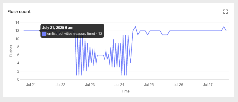
Debugging high latency
If your pipeline latency is higher than expected, use the “Flush Count” graph in the analytics portal to identify which condition is triggering flushes —size, rows, or time — then adjust accordingly.
- OLAP destinations
- OLTP destinations
Check the flush reason
Look at the “Flush Count” graph to see which condition is triggering flushes.
If the reason is size or rows
Your flushes are triggering before enough data accumulates, producing small batches with high per-row overhead. Increase the limits toward the upper end of the recommended range:
- Rows: increase toward 500k
- Bytes: increase toward 500 MB
Monitoring
You can see which flush rule triggered each flush in the analytics portal: